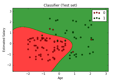
Kernel SVM Intuitioin
Data Type:
– Linearly Separable
– Not Linearly Separable => Kernel SVM
A Higher-Dimensional Space
Mapping to a higher dimension.
[1D Space] (x1)
f = x -5
[2D Space] (x1, x2)
f = (x -5)^2
[3D Space] (x1, x2, z)
=> can be highly compute-intensive.
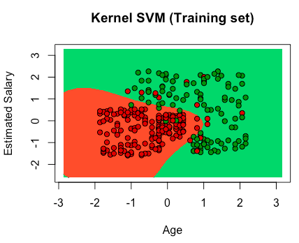
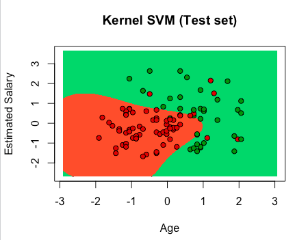
The Gaussian RBF Kernel
Types of Kernel Functions
– Gaussian RBF Kernel
K(x→,l→i) = e -(||x→-l→i||2) / 2σ2
– Sigmoid Kernel
K(X,Y) = tanh(γ・XTY + r)
– Polynomial Kernel
K(X,Y) = (γ・XTY + r)d,γ>0
http://mlkernels.readthedocs.io/en/latest/kernels.html
(http://mlkernels.readthedocs.io/en/latest/kernelfunctions.html)
Implementation
Python
1 2 3 4 5 6 7 8 9 10 11 12 13 14 15 16 17 18 19 20 21 22 23 24 25 26 27 28 29 30 31 32 33 34 35 36 37 38 39 40 41 42 43 44 45 46 47 48 49 50 51 52 53 54 55 56 57 58 59 60 61 62 63 64 65 66 67 68 69 |
# Kernel SVM # Importing the libraries import numpy as np import matplotlib.pyplot as plt import pandas as pd # Importing the dataset dataset = pd.read_csv('Social_Network_Ads.csv') X = dataset.iloc[:, [2, 3]].values y = dataset.iloc[:, 4].values # Splitting the dataset into the Training set and Test set from sklearn.cross_validation import train_test_split X_train, X_test, y_train, y_test = train_test_split(X, y, test_size = 0.25, random_state = 0) # Feature Scaling from sklearn.preprocessing import StandardScaler sc = StandardScaler() X_train = sc.fit_transform(X_train) X_test = sc.transform(X_test) # Fitting classifier to the Training set from sklearn.svm import SVC classifier = SVC(kernel = 'rbf', random_state = 0) classifier.fit(X_train, y_train) # Predicting the Test set results y_pred = classifier.predict(X_test) # Making the Confusion Matrix from sklearn.metrics import confusion_matrix cm = confusion_matrix(y_test, y_pred) # Visualising the Training set results from matplotlib.colors import ListedColormap X_set, y_set = X_train, y_train X1, X2 = np.meshgrid(np.arange(start = X_set[:, 0].min() - 1, stop = X_set[:, 0].max() + 1, step = 0.01), np.arange(start = X_set[:, 1].min() - 1, stop = X_set[:, 1].max() + 1, step = 0.01)) plt.contourf(X1, X2, classifier.predict(np.array([X1.ravel(), X2.ravel()]).T).reshape(X1.shape), alpha = 0.75, cmap = ListedColormap(('red', 'green'))) plt.xlim(X1.min(), X1.max()) plt.ylim(X2.min(), X2.max()) for i, j in enumerate(np.unique(y_set)): plt.scatter(X_set[y_set == j, 0], X_set[y_set == j, 1], c = ListedColormap(('red', 'green'))(i), label = j) plt.title('Classifier (Training set)') plt.xlabel('Age') plt.ylabel('Estimated Salary') plt.legend() plt.show() # Visualising the Test set results from matplotlib.colors import ListedColormap X_set, y_set = X_test, y_test X1, X2 = np.meshgrid(np.arange(start = X_set[:, 0].min() - 1, stop = X_set[:, 0].max() + 1, step = 0.01), np.arange(start = X_set[:, 1].min() - 1, stop = X_set[:, 1].max() + 1, step = 0.01)) plt.contourf(X1, X2, classifier.predict(np.array([X1.ravel(), X2.ravel()]).T).reshape(X1.shape), alpha = 0.75, cmap = ListedColormap(('red', 'green'))) plt.xlim(X1.min(), X1.max()) plt.ylim(X2.min(), X2.max()) for i, j in enumerate(np.unique(y_set)): plt.scatter(X_set[y_set == j, 0], X_set[y_set == j, 1], c = ListedColormap(('red', 'green'))(i), label = j) plt.title('Classifier (Test set)') plt.xlabel('Age') plt.ylabel('Estimated Salary') plt.legend() plt.show() |

R
1 2 3 4 5 6 7 8 9 10 11 12 13 14 15 16 17 18 19 20 21 22 23 24 25 26 27 28 29 30 31 32 33 34 35 36 37 38 39 40 41 42 43 44 45 46 47 48 49 50 51 52 53 54 55 56 57 58 59 60 61 62 63 64 65 |
# Kernel SVM # Importing the dataset dataset = read.csv('Social_Network_Ads.csv') dataset = dataset[3:5] # Encoding the target feature as factor dataset$Purchased = factor(dataset$Purchased, levels = c(0, 1)) # Splitting the dataset into the Training set and Test set # install.packages('caTools') library(caTools) set.seed(123) split = sample.split(dataset$Purchased, SplitRatio = 0.75) training_set = subset(dataset, split == TRUE) test_set = subset(dataset, split == FALSE) # Feature Scaling training_set[-3] = scale(training_set[-3]) test_set[-3] = scale(test_set[-3]) # Fitting classifier to the Training set # install.packages('e1071') library(e1071) classifier = svm(formula = Purchased ~ ., data = training_set, type = 'C-classification', kernel = 'radial') # Predicting the Test set results y_pred = predict(classifier, newdata = test_set[-3]) # Making the Confusion Matrix cm = table(test_set[, 3], y_pred) # Visualising the Training set results library(ElemStatLearn) set = training_set X1 = seq(min(set[, 1]) - 1, max(set[, 1]) + 1, by = 0.01) X2 = seq(min(set[, 2]) - 1, max(set[, 2]) + 1, by = 0.01) grid_set = expand.grid(X1, X2) colnames(grid_set) = c('Age', 'EstimatedSalary') y_grid = predict(classifier, newdata = grid_set) plot(set[, -3], main = 'Kernel SVM (Training set)', xlab = 'Age', ylab = 'Estimated Salary', xlim = range(X1), ylim = range(X2)) contour(X1, X2, matrix(as.numeric(y_grid), length(X1), length(X2)), add = TRUE) points(grid_set, pch = '.', col = ifelse(y_grid == 1, 'springgreen3', 'tomato')) points(set, pch = 21, bg = ifelse(set[, 3] == 1, 'green4', 'red3')) # Visualising the Test set results library(ElemStatLearn) set = test_set X1 = seq(min(set[, 1]) - 1, max(set[, 1]) + 1, by = 0.01) X2 = seq(min(set[, 2]) - 1, max(set[, 2]) + 1, by = 0.01) grid_set = expand.grid(X1, X2) colnames(grid_set) = c('Age', 'EstimatedSalary') y_grid = predict(classifier, newdata = grid_set) plot(set[, -3], main = 'Kernel SVM (Test set)', xlab = 'Age', ylab = 'Estimated Salary', xlim = range(X1), ylim = range(X2)) contour(X1, X2, matrix(as.numeric(y_grid), length(X1), length(X2)), add = TRUE) points(grid_set, pch = '.', col = ifelse(y_grid == 1, 'springgreen3', 'tomato')) points(set, pch = 21, bg = ifelse(set[, 3] == 1, 'green4', 'red3')) |
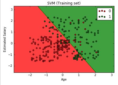
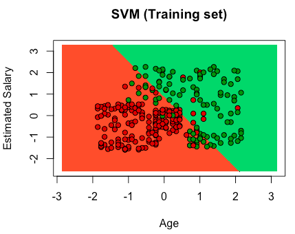
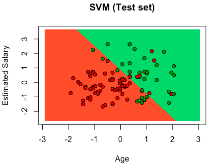
Support Vector Machine (SVM)
classification: how to classify added new data point.
Maximum Margin: a margin which has maximized space between support vectors.
Support Vectors: vectors which decides the maximum margin.
Maximum Margin Hyperplane (Maximum Margin Classifier)
Positive Hyperplane
Negative Hyperplane
Implementation
Python
1 2 3 4 5 6 7 8 9 10 11 12 13 14 15 16 17 18 19 20 21 22 23 24 25 26 27 28 29 30 31 32 33 34 35 36 37 38 39 40 41 42 43 44 45 46 47 48 49 50 51 52 53 54 55 56 57 58 59 60 61 62 63 64 65 66 67 68 69 |
# Support Vector Machine (SVM) # Importing the libraries import numpy as np import matplotlib.pyplot as plt import pandas as pd # Importing the dataset dataset = pd.read_csv('Social_Network_Ads.csv') X = dataset.iloc[:, [2, 3]].values y = dataset.iloc[:, 4].values # Splitting the dataset into the Training set and Test set from sklearn.cross_validation import train_test_split X_train, X_test, y_train, y_test = train_test_split(X, y, test_size = 0.25, random_state = 0) # Feature Scaling from sklearn.preprocessing import StandardScaler sc = StandardScaler() X_train = sc.fit_transform(X_train) X_test = sc.transform(X_test) # Fitting SVM to the Training set from sklearn.svm import SVC classifier = SVC(kernel = 'linear', random_state = 0) classifier.fit(X_train, y_train) # Predicting the Test set results y_pred = classifier.predict(X_test) # Making the Confusion Matrix from sklearn.metrics import confusion_matrix cm = confusion_matrix(y_test, y_pred) # Visualising the Training set results from matplotlib.colors import ListedColormap X_set, y_set = X_train, y_train X1, X2 = np.meshgrid(np.arange(start = X_set[:, 0].min() - 1, stop = X_set[:, 0].max() + 1, step = 0.01), np.arange(start = X_set[:, 1].min() - 1, stop = X_set[:, 1].max() + 1, step = 0.01)) plt.contourf(X1, X2, classifier.predict(np.array([X1.ravel(), X2.ravel()]).T).reshape(X1.shape), alpha = 0.75, cmap = ListedColormap(('red', 'green'))) plt.xlim(X1.min(), X1.max()) plt.ylim(X2.min(), X2.max()) for i, j in enumerate(np.unique(y_set)): plt.scatter(X_set[y_set == j, 0], X_set[y_set == j, 1], c = ListedColormap(('red', 'green'))(i), label = j) plt.title('SVM (Training set)') plt.xlabel('Age') plt.ylabel('Estimated Salary') plt.legend() plt.show() # Visualising the Test set results from matplotlib.colors import ListedColormap X_set, y_set = X_test, y_test X1, X2 = np.meshgrid(np.arange(start = X_set[:, 0].min() - 1, stop = X_set[:, 0].max() + 1, step = 0.01), np.arange(start = X_set[:, 1].min() - 1, stop = X_set[:, 1].max() + 1, step = 0.01)) plt.contourf(X1, X2, classifier.predict(np.array([X1.ravel(), X2.ravel()]).T).reshape(X1.shape), alpha = 0.75, cmap = ListedColormap(('red', 'green'))) plt.xlim(X1.min(), X1.max()) plt.ylim(X2.min(), X2.max()) for i, j in enumerate(np.unique(y_set)): plt.scatter(X_set[y_set == j, 0], X_set[y_set == j, 1], c = ListedColormap(('red', 'green'))(i), label = j) plt.title('SVM (Test set)') plt.xlabel('Age') plt.ylabel('Estimated Salary') plt.legend() plt.show() |

R
1 2 3 4 5 6 7 8 9 10 11 12 13 14 15 16 17 18 19 20 21 22 23 24 25 26 27 28 29 30 31 32 33 34 35 36 37 38 39 40 41 42 43 44 45 46 47 48 49 50 51 52 53 54 55 56 57 58 59 60 61 62 63 64 |
# Support Vector Machine (SVM) # Importing the dataset dataset = read.csv('Social_Network_Ads.csv') dataset = dataset[3:5] # Encoding the target feature as factor dataset$Purchased = factor(dataset$Purchased, levels = c(0, 1)) # Splitting the dataset into the Training set and Test set # install.packages('caTools') library(caTools) set.seed(123) split = sample.split(dataset$Purchased, SplitRatio = 0.75) training_set = subset(dataset, split == TRUE) test_set = subset(dataset, split == FALSE) # Feature Scaling training_set[-3] = scale(training_set[-3]) test_set[-3] = scale(test_set[-3]) # Fitting classifier to the Training set library(e1071) classifier = svm(formula = Purchased ~ ., data = training_set, type = 'C-classification', kernel = 'linear') # Predicting the Test set results y_pred = predict(classifier, newdata = test_set[-3]) # Making the Confusion Matrix cm = table(test_set[, 3], y_pred) # Visualising the Training set results library(ElemStatLearn) set = training_set X1 = seq(min(set[, 1]) - 1, max(set[, 1]) + 1, by = 0.01) X2 = seq(min(set[, 2]) - 1, max(set[, 2]) + 1, by = 0.01) grid_set = expand.grid(X1, X2) colnames(grid_set) = c('Age', 'EstimatedSalary') y_grid = predict(classifier, newdata = grid_set) plot(set[, -3], main = 'Classifier (Training set)', xlab = 'Age', ylab = 'Estimated Salary', xlim = range(X1), ylim = range(X2)) contour(X1, X2, matrix(as.numeric(y_grid), length(X1), length(X2)), add = TRUE) points(grid_set, pch = '.', col = ifelse(y_grid == 1, 'springgreen3', 'tomato')) points(set, pch = 21, bg = ifelse(set[, 3] == 1, 'green4', 'red3')) # Visualising the Test set results library(ElemStatLearn) set = test_set X1 = seq(min(set[, 1]) - 1, max(set[, 1]) + 1, by = 0.01) X2 = seq(min(set[, 2]) - 1, max(set[, 2]) + 1, by = 0.01) grid_set = expand.grid(X1, X2) colnames(grid_set) = c('Age', 'EstimatedSalary') y_grid = predict(classifier, newdata = grid_set) plot(set[, -3], main = 'Classifier (Test set)', xlab = 'Age', ylab = 'Estimated Salary', xlim = range(X1), ylim = range(X2)) contour(X1, X2, matrix(as.numeric(y_grid), length(X1), length(X2)), add = TRUE) points(grid_set, pch = '.', col = ifelse(y_grid == 1, 'springgreen3', 'tomato')) points(set, pch = 21, bg = ifelse(set[, 3] == 1, 'green4', 'red3')) |
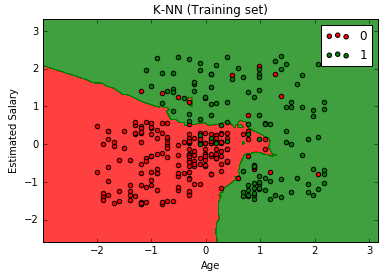
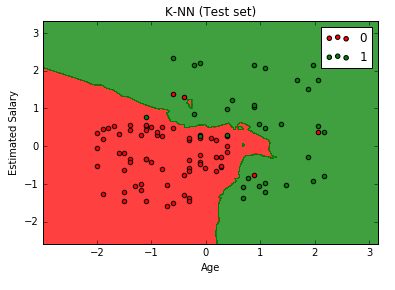
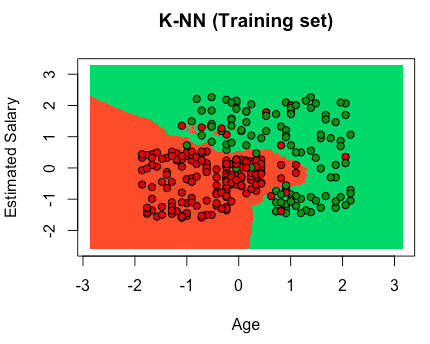
K-NN Intuition
How do we classify a new data point between category 1 and 2?
K-NN identifies which category the new data point should be in.
STEP 1: Choose the number K of neighbors
STEP 2: Take the K nearest neighbors of the new data point, according to the Euclidean distance
STEP 3: Among these K neighbors, count the number of data points in each category
STEP 4: Assign the new data point to the category where you counted the most neighbors
Euclidean Distance
2 points:
P1(x1, y1)
P2(x2, y2)
Euclidean Distance between P1 and P2 = √((x2 – x1)2 + (y2 – y1)2)
Implementation
Python
1 2 3 4 5 6 7 8 9 10 11 12 13 14 15 16 17 18 19 20 21 22 23 24 25 26 27 28 29 30 31 32 33 34 35 36 37 38 39 40 41 42 43 44 45 46 47 48 49 50 51 52 53 54 55 56 57 58 59 60 61 62 63 64 65 66 67 68 69 |
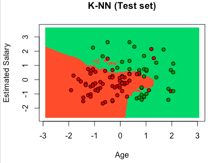
# K-Nearest Neighbors (K-NN) # Importing the libraries import numpy as np import matplotlib.pyplot as plt import pandas as pd # Importing the dataset dataset = pd.read_csv('Social_Network_Ads.csv') X = dataset.iloc[:, [2,3]].values y = dataset.iloc[:, 4].values # Splitting the dataset into the Training set and Test set from sklearn.cross_validation import train_test_split X_train, X_test, y_train, y_test = train_test_split(X, y, test_size = 0.25, random_state = 0) # Feature Scaling from sklearn.preprocessing import StandardScaler sc_X = StandardScaler() X_train = sc_X.fit_transform(X_train) X_test = sc_X.transform(X_test) # Fitting the classifier to the dataset from sklearn.neighbors import KNeighborsClassifier classifier = KNeighborsClassifier(n_neighbors = 5, metric = 'minkowski', p = 2) classifier.fit(X_train, y_train) # Predicting a new result y_pred = classifier.predict(X_test) # Making the Confusion Matrix from sklearn.metrics import confusion_matrix cm = confusion_matrix(y_test, y_pred) # Visualizing the Training set results from matplotlib.colors import ListedColormap X_set, y_set = X_train, y_train X1, X2 = np.meshgrid(np.arange(start = X_set[:, 0].min() - 1, stop = X_set[:, 0].max() + 1, step = 0.01), np.arange(start = X_set[:, 1].min() - 1, stop = X_set[:, 1].max() + 1, step = 0.01)) plt.contourf(X1, X2, classifier.predict(np.array([X1.ravel(), X2.ravel()]).T).reshape(X1.shape), alpha = 0.75, cmap = ListedColormap(('red', 'green'))) plt.xlim(X1.min(), X1.max()) plt.ylim(X2.min(), X2.max()) for i, j in enumerate(np.unique(y_set)): plt.scatter(X_set[y_set == j, 0], X_set[y_set == j, 1], c = ListedColormap(('red', 'green'))(i), label = j) plt.title('K-NN (Training set)') plt.xlabel('Age') plt.ylabel('Estimated Salary') plt.legend() plt.show() # Visualizing the Test set results from matplotlib.colors import ListedColormap X_set, y_set = X_test, y_test X1, X2 = np.meshgrid(np.arange(start = X_set[:, 0].min() - 1, stop = X_set[:, 0].max() + 1, step = 0.01), np.arange(start = X_set[:, 1].min() - 1, stop = X_set[:, 1].max() + 1, step = 0.01)) plt.contourf(X1, X2, classifier.predict(np.array([X1.ravel(), X2.ravel()]).T).reshape(X1.shape), alpha = 0.75, cmap = ListedColormap(('red', 'green'))) plt.xlim(X1.min(), X1.max()) plt.ylim(X2.min(), X2.max()) for i, j in enumerate(np.unique(y_set)): plt.scatter(X_set[y_set == j, 0], X_set[y_set == j, 1], c = ListedColormap(('red', 'green'))(i), label = j) plt.title('K-NN (Test set)') plt.xlabel('Age') plt.ylabel('Estimated Salary') plt.legend() plt.show() |
R
1 2 3 4 5 6 7 8 9 10 11 12 13 14 15 16 17 18 19 20 21 22 23 24 25 26 27 28 29 30 31 32 33 34 35 36 37 38 39 40 41 42 43 44 45 46 47 48 49 50 51 52 53 54 55 56 57 58 59 60 61 62 63 64 65 66 67 68 69 70 |
# K-Nearest Neighbors (K-NN) # Importing the dataset dataset = read.csv('Social_Network_Ads.csv') dataset = dataset[3:5] # Encoding the target feature as factor dataset$Purchased = factor(dataset$Purchased, levels = c(0,1)) # Splitting the dataset into the Training set and Test set # install.packages('caTools') library(caTools) set.seed(123) split = sample.split(dataset$Purchased, SplitRatio = 0.75) training_set = subset(dataset, split == TRUE) test_set = subset(dataset, split == FALSE) # Feature Scaling training_set[-3] = scale(training_set[-3]) test_set[-3] = scale(test_set[-3]) # Fitting K-NN to the Training set and predicting the Test set results library(class) y_pred = knn(train = training_set[, -3], test = test_set[, -3], cl = training_set[, 3], k = 5) # Making the Confusion Matrix cm = table(test_set[, 3], y_pred) # Visualising the Training set results # install.packages('ElemStatLearn') library(ElemStatLearn) set = training_set X1 = seq(min(set[, 1]) - 1, max(set[, 1]) + 1, by = 0.01) X2 = seq(min(set[, 2]) - 1, max(set[, 2]) + 1, by = 0.01) grid_set = expand.grid(X1, X2) colnames(grid_set) = c('Age', 'EstimatedSalary') y_grid = knn(train = training_set[, -3], test = grid_set, cl = training_set[, 3], k = 5) plot(set[, -3], main = 'K-NN (Training set)', xlab = 'Age', ylab = 'Estimated Salary', xlim = range(X1), ylim = range(X2)) contour(X1, X2, matrix(as.numeric(y_grid), length(X1), length(X2)), add = TRUE) points(grid_set, pch = '.', col = ifelse(y_grid == 1, 'springgreen3', 'tomato')) points(set, pch = 21, bg = ifelse(set[, 3] == 1, 'green4', 'red3')) # Visualising the Test set results # install.packages('ElemStatLearn') # library(ElemStatLearn) set = test_set X1 = seq(min(set[, 1]) - 1, max(set[, 1]) + 1, by = 0.01) X2 = seq(min(set[, 2]) - 1, max(set[, 2]) + 1, by = 0.01) grid_set = expand.grid(X1, X2) colnames(grid_set) = c('Age', 'EstimatedSalary') y_grid = knn(train = training_set[, -3], test = grid_set, cl = training_set[, 3], k = 5) plot(set[, -3], main = 'K-NN (Test set)', xlab = 'Age', ylab = 'Estimated Salary', xlim = range(X1), ylim = range(X2)) contour(X1, X2, matrix(as.numeric(y_grid), length(X1), length(X2)), add = TRUE) points(grid_set, pch = '.', col = ifelse(y_grid == 1, 'springgreen3', 'tomato')) points(set, pch = 21, bg = ifelse(set[, 3] == 1, 'green4', 'red3')) |
Linear Regression
– Simple:
y = b0 + b1 * x1
– Multiple:
y = b0 + b1 * x1 + … + bn * xn
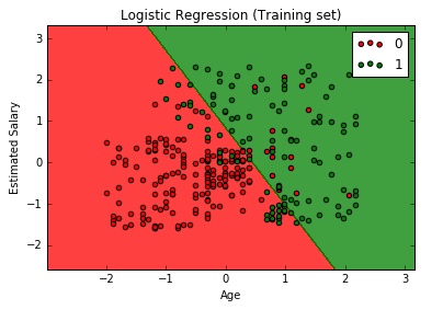
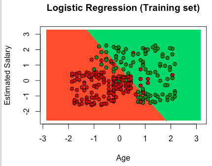
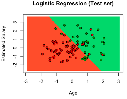
Logistic Regression
Sigmoid Function:
p = 1 / (1 + e-y)
ln * (p / (1 – p)) = b0 + b1 * x
y: Actual DV [dependent variable]
p^: Probability [p_hat]
y^: Predicted DV
Implementation
Python
1 2 3 4 5 6 7 8 9 10 11 12 13 14 15 16 17 18 19 20 21 22 23 24 25 26 27 28 29 30 31 32 33 34 35 36 37 38 39 40 41 42 43 44 45 46 47 48 49 50 51 52 53 54 55 56 57 58 59 60 61 62 63 64 |
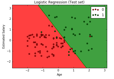
# Logistic Regression # Importing the dataset dataset = pd.read_csv('Social_Network_Ads.csv') X = dataset.iloc[:, [2,3]].values y = dataset.iloc[:, 4].values # Splitting the dataset into the Training set and Test set from sklearn.cross_validation import train_test_split X_train, X_test, y_train, y_test = train_test_split(X, y, test_size = 0.25, random_state = 0) # Feature Scaling from sklearn.preprocessing import StandardScaler sc_X = StandardScaler() X_train = sc_X.fit_transform(X_train) X_test = sc_X.transform(X_test) # Fitting the Regression to the dataset from sklearn.linear_model import LogisticRegression classifier = LogisticRegression(random_state = 0) classifier.fit(X_train, y_train) # Predicting a new result y_pred = classifier.predict(X_test) # Making the Confusion Matrix from sklearn.metrics import confusion_matrix cm = confusion_matrix(y_test, y_pred) # Visualizing the Training set results from matplotlib.colors import ListedColormap X_set, y_set = X_train, y_train X1, X2 = np.meshgrid(np.arange(start = X_set[:, 0].min() - 1, stop = X_set[:, 0].max() + 1, step = 0.01), np.arange(start = X_set[:, 1].min() - 1, stop = X_set[:, 1].max() + 1, step = 0.01)) plt.contourf(X1, X2, classifier.predict(np.array([X1.ravel(), X2.ravel()]).T).reshape(X1.shape), alpha = 0.75, cmap = ListedColormap(('red', 'green'))) plt.xlim(X1.min(), X1.max()) plt.ylim(X2.min(), X2.max()) for i, j in enumerate(np.unique(y_set)): plt.scatter(X_set[y_set == j, 0], X_set[y_set == j, 1], c = ListedColormap(('red', 'green'))(i), label = j) plt.title('Logistic Regression (Training set)') plt.xlabel('Age') plt.ylabel('Estimated Salary') plt.legend() plt.show() # Visualizing the Test set results from matplotlib.colors import ListedColormap X_set, y_set = X_test, y_test X1, X2 = np.meshgrid(np.arange(start = X_set[:, 0].min() - 1, stop = X_set[:, 0].max() + 1, step = 0.01), np.arange(start = X_set[:, 1].min() - 1, stop = X_set[:, 1].max() + 1, step = 0.01)) plt.contourf(X1, X2, classifier.predict(np.array([X1.ravel(), X2.ravel()]).T).reshape(X1.shape), alpha = 0.75, cmap = ListedColormap(('red', 'green'))) plt.xlim(X1.min(), X1.max()) plt.ylim(X2.min(), X2.max()) for i, j in enumerate(np.unique(y_set)): plt.scatter(X_set[y_set == j, 0], X_set[y_set == j, 1], c = ListedColormap(('red', 'green'))(i), label = j) plt.title('Logistic Regression (Test set)') plt.xlabel('Age') plt.ylabel('Estimated Salary') plt.legend() plt.show() |
R
1 2 3 4 5 6 7 8 9 10 11 12 13 14 15 16 17 18 19 20 21 22 23 24 25 26 27 28 29 30 31 32 33 34 35 36 37 38 39 40 41 42 43 44 45 46 47 48 49 50 51 52 53 54 55 56 57 58 59 60 61 62 63 64 65 |
# Logistic Regression # Importing the dataset dataset = read.csv('Social_Network_Ads.csv') dataset = dataset[, 3:5] # Splitting the dataset into the Training set and Test set # install.packages('caTools') library(caTools) set.seed(123) split = sample.split(dataset$Purchased, SplitRatio = 0.75) training_set = subset(dataset, split == TRUE) test_set = subset(dataset, split == FALSE) # Feature Scaling training_set[, 1:2] = scale(training_set[, 1:2]) test_set[, 1:2] = scale(test_set[, 1:2]) # Fitting Logistic Regression to the Training set classifier = glm(formula = Purchased ~ ., family = binomial, data = training_set) # Predicting the Test set results prob_pred = predict(classifier, type = 'response', newdata = test_set[-3]) y_pred = ifelse(prob_pred > 0.5, 1, 0) # Making the Confusion Matrix cm = table(test_set[, 3], y_pred) # Visualising the Training set results # install.packages('ElemStatLearn') library(ElemStatLearn) set = training_set X1 = seq(min(set[, 1]) - 1, max(set[, 1]) + 1, by = 0.01) X2 = seq(min(set[, 2]) - 1, max(set[, 2]) + 1, by = 0.01) grid_set = expand.grid(X1, X2) colnames(grid_set) = c('Age', 'EstimatedSalary') prob_set = predict(classifier, type = 'response', newdata = grid_set) y_grid = ifelse(prob_set > 0.5, 1, 0) plot(set[, -3], main = 'Logistic Regression (Training set)', xlab = 'Age', ylab = 'Estimated Salary', xlim = range(X1), ylim = range(X2)) contour(X1, X2, matrix(as.numeric(y_grid), length(X1), length(X2)), add = TRUE) points(grid_set, pch = '.', col = ifelse(y_grid == 1, 'springgreen3', 'tomato')) points(set, pch = 21, bg = ifelse(set[, 3] == 1, 'green4', 'red3')) # Visualising the Test set results # install.packages('ElemStatLearn') # library(ElemStatLearn) set = test_set X1 = seq(min(set[, 1]) - 1, max(set[, 1]) + 1, by = 0.01) X2 = seq(min(set[, 2]) - 1, max(set[, 2]) + 1, by = 0.01) grid_set = expand.grid(X1, X2) colnames(grid_set) = c('Age', 'EstimatedSalary') prob_set = predict(classifier, type = 'response', newdata = grid_set) y_grid = ifelse(prob_set > 0.5, 1, 0) plot(set[, -3], main = 'Logistic Regression (Test set)', xlab = 'Age', ylab = 'Estimated Salary', xlim = range(X1), ylim = range(X2)) contour(X1, X2, matrix(as.numeric(y_grid), length(X1), length(X2)), add = TRUE) points(grid_set, pch = '.', col = ifelse(y_grid == 1, 'springgreen3', 'tomato')) points(set, pch = 21, bg = ifelse(set[, 3] == 1, 'green4', 'red3')) |
Templates
Python
1 2 3 4 5 6 7 8 9 10 11 12 13 14 15 16 17 18 19 20 21 22 23 24 25 26 27 28 29 30 31 32 33 34 35 36 37 38 39 40 41 42 43 44 45 46 47 48 49 50 51 52 53 54 55 56 57 58 59 60 61 62 63 64 65 66 67 |
# Classification Template # Importing the libraries import numpy as np import matplotlib.pyplot as plt import pandas as pd # Importing the dataset dataset = pd.read_csv('Social_Network_Ads.csv') X = dataset.iloc[:, [2,3]].values y = dataset.iloc[:, 4].values # Splitting the dataset into the Training set and Test set from sklearn.cross_validation import train_test_split X_train, X_test, y_train, y_test = train_test_split(X, y, test_size = 0.25, random_state = 0) # Feature Scaling from sklearn.preprocessing import StandardScaler sc_X = StandardScaler() X_train = sc_X.fit_transform(X_train) X_test = sc_X.transform(X_test) # Fitting the classifier to the dataset # Create your classifier here # Predicting a new result y_pred = classifier.predict(X_test) # Making the Confusion Matrix from sklearn.metrics import confusion_matrix cm = confusion_matrix(y_test, y_pred) # Visualizing the Training set results from matplotlib.colors import ListedColormap X_set, y_set = X_train, y_train X1, X2 = np.meshgrid(np.arange(start = X_set[:, 0].min() - 1, stop = X_set[:, 0].max() + 1, step = 0.01), np.arange(start = X_set[:, 1].min() - 1, stop = X_set[:, 1].max() + 1, step = 0.01)) plt.contourf(X1, X2, classifier.predict(np.array([X1.ravel(), X2.ravel()]).T).reshape(X1.shape), alpha = 0.75, cmap = ListedColormap(('red', 'green'))) plt.xlim(X1.min(), X1.max()) plt.ylim(X2.min(), X2.max()) for i, j in enumerate(np.unique(y_set)): plt.scatter(X_set[y_set == j, 0], X_set[y_set == j, 1], c = ListedColormap(('red', 'green'))(i), label = j) plt.title('Logistic Regression (Training set)') plt.xlabel('Age') plt.ylabel('Estimated Salary') plt.legend() plt.show() # Visualizing the Test set results from matplotlib.colors import ListedColormap X_set, y_set = X_test, y_test X1, X2 = np.meshgrid(np.arange(start = X_set[:, 0].min() - 1, stop = X_set[:, 0].max() + 1, step = 0.01), np.arange(start = X_set[:, 1].min() - 1, stop = X_set[:, 1].max() + 1, step = 0.01)) plt.contourf(X1, X2, classifier.predict(np.array([X1.ravel(), X2.ravel()]).T).reshape(X1.shape), alpha = 0.75, cmap = ListedColormap(('red', 'green'))) plt.xlim(X1.min(), X1.max()) plt.ylim(X2.min(), X2.max()) for i, j in enumerate(np.unique(y_set)): plt.scatter(X_set[y_set == j, 0], X_set[y_set == j, 1], c = ListedColormap(('red', 'green'))(i), label = j) plt.title('Logistic Regression (Test set)') plt.xlabel('Age') plt.ylabel('Estimated Salary') plt.legend() plt.show() |
R
1 2 3 4 5 6 7 8 9 10 11 12 13 14 15 16 17 18 19 20 21 22 23 24 25 26 27 28 29 30 31 32 33 34 35 36 37 38 39 40 41 42 43 44 45 46 47 48 49 50 51 52 53 54 55 56 57 58 59 60 61 62 63 64 65 66 |
# Classification Template # Importing the dataset dataset = read.csv('Social_Network_Ads.csv') dataset = dataset[3:5] # Encoding the target feature as factor dataset$Purchased = factor(dataset$Purchased, levels = c(0,1)) # Splitting the dataset into the Training set and Test set # install.packages('caTools') library(caTools) set.seed(123) split = sample.split(dataset$Purchased, SplitRatio = 0.75) training_set = subset(dataset, split == TRUE) test_set = subset(dataset, split == FALSE) # Feature Scaling training_set[-3] = scale(training_set[-3]) test_set[-3] = scale(test_set[-3]) # Fitting classifier to the Training set # Create your classifier here # Predicting the Test set results prob_pred = predict(classifier, type = 'response', newdata = test_set[-3]) y_pred = ifelse(prob_pred > 0.5, 1, 0) # Making the Confusion Matrix cm = table(test_set[, 3], y_pred > 0.5) # Visualising the Training set results # install.packages('ElemStatLearn') library(ElemStatLearn) set = training_set X1 = seq(min(set[, 1]) - 1, max(set[, 1]) + 1, by = 0.01) X2 = seq(min(set[, 2]) - 1, max(set[, 2]) + 1, by = 0.01) grid_set = expand.grid(X1, X2) colnames(grid_set) = c('Age', 'EstimatedSalary') prob_set = predict(classifier, type = 'response', newdata = grid_set) y_grid = ifelse(prob_set > 0.5, 1, 0) plot(set[, -3], main = 'Classifier (Training set)', xlab = 'Age', ylab = 'Estimated Salary', xlim = range(X1), ylim = range(X2)) contour(X1, X2, matrix(as.numeric(y_grid), length(X1), length(X2)), add = TRUE) points(grid_set, pch = '.', col = ifelse(y_grid == 1, 'springgreen3', 'tomato')) points(set, pch = 21, bg = ifelse(set[, 3] == 1, 'green4', 'red3')) # Visualising the Test set results # install.packages('ElemStatLearn') # library(ElemStatLearn) set = test_set X1 = seq(min(set[, 1]) - 1, max(set[, 1]) + 1, by = 0.01) X2 = seq(min(set[, 2]) - 1, max(set[, 2]) + 1, by = 0.01) grid_set = expand.grid(X1, X2) colnames(grid_set) = c('Age', 'EstimatedSalary') prob_set = predict(classifier, type = 'response', newdata = grid_set) y_grid = ifelse(prob_set > 0.5, 1, 0) plot(set[, -3], main = 'Classifier (Test set)', xlab = 'Age', ylab = 'Estimated Salary', xlim = range(X1), ylim = range(X2)) contour(X1, X2, matrix(as.numeric(y_grid), length(X1), length(X2)), add = TRUE) points(grid_set, pch = '.', col = ifelse(y_grid == 1, 'springgreen3', 'tomato')) points(set, pch = 21, bg = ifelse(set[, 3] == 1, 'green4', 'red3')) |
R Squared Intuition
Simple Linear Regression
R Squared
SUM (yi – yi^)2 -> min
SSres = SUM (yi – yi^)2
res = residual
SStot = SUM (yi – yavg)2
tot = total
R2 = 1 – SSres / SStot
Adjusted R2 (R Squared)
R2 = 1 – SSres / SStot
y = b0 + b1 * x1
y = b0 + b1 * x1 + b2 * x2
SSres -> Min
R2 – Goodness of fit (greater is better)
Problem:
y = b0 + b1 * x1 + b2 * x2 (+ b3 * x3)
SSres -> Min
R2 will never decrease
R2 = 1 – SSres / SStot
Adj R2 = 1 – (1 – R2) * (n-1) / (n- p – 1)
p – number of regressors
n – sample size
1. Pros and cons of each regression model
https://www.superdatascience.com/wp-content/uploads/2017/02/Regression-Pros-Cons.pdf
2. How do I know which model to choose for my problem ?
1) Figure out whether your problem is linear or non linear.
– linear:
– only one feature: Simple Linear Regression
– several features: Multiple Linear Regression
– non linear:
– Polynomial Regression
– SVR
– Decision Tree
– Random Forest
3. How can I improve each of these models ?
=> In Part 10 – Model Selection
a. The parameters that are learnt, for example the coefficients in Linear Regression.
b. The hyperparameters.
– not learnt
– fixed values inside the model equations.
https://www.superdatascience.com/wp-content/uploads/2017/02/Regularization.pdf