Machine Learning A-Z: Part 3 – Classification (Kernel SVM Intuitioin)
Kernel SVM Intuitioin
Data Type:
– Linearly Separable
– Not Linearly Separable => Kernel SVM
A Higher-Dimensional Space
Mapping to a higher dimension.
[1D Space] (x1)
f = x -5
[2D Space] (x1, x2)
f = (x -5)^2
[3D Space] (x1, x2, z)
=> can be highly compute-intensive.
The Gaussian RBF Kernel
Types of Kernel Functions
– Gaussian RBF Kernel
K(x→,l→i) = e -(||x→-l→i||2) / 2σ2
– Sigmoid Kernel
K(X,Y) = tanh(γ・XTY + r)
– Polynomial Kernel
K(X,Y) = (γ・XTY + r)d,γ>0
http://mlkernels.readthedocs.io/en/latest/kernels.html
(http://mlkernels.readthedocs.io/en/latest/kernelfunctions.html)
Implementation
Python
|
1 2 3 4 5 6 7 8 9 10 11 12 13 14 15 16 17 18 19 20 21 22 23 24 25 26 27 28 29 30 31 32 33 34 35 36 37 38 39 40 41 42 43 44 45 46 47 48 49 50 51 52 53 54 55 56 57 58 59 60 61 62 63 64 65 66 67 68 69 |
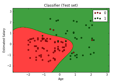
# Kernel SVM # Importing the libraries import numpy as np import matplotlib.pyplot as plt import pandas as pd # Importing the dataset dataset = pd.read_csv('Social_Network_Ads.csv') X = dataset.iloc[:, [2, 3]].values y = dataset.iloc[:, 4].values # Splitting the dataset into the Training set and Test set from sklearn.cross_validation import train_test_split X_train, X_test, y_train, y_test = train_test_split(X, y, test_size = 0.25, random_state = 0) # Feature Scaling from sklearn.preprocessing import StandardScaler sc = StandardScaler() X_train = sc.fit_transform(X_train) X_test = sc.transform(X_test) # Fitting classifier to the Training set from sklearn.svm import SVC classifier = SVC(kernel = 'rbf', random_state = 0) classifier.fit(X_train, y_train) # Predicting the Test set results y_pred = classifier.predict(X_test) # Making the Confusion Matrix from sklearn.metrics import confusion_matrix cm = confusion_matrix(y_test, y_pred) # Visualising the Training set results from matplotlib.colors import ListedColormap X_set, y_set = X_train, y_train X1, X2 = np.meshgrid(np.arange(start = X_set[:, 0].min() - 1, stop = X_set[:, 0].max() + 1, step = 0.01), np.arange(start = X_set[:, 1].min() - 1, stop = X_set[:, 1].max() + 1, step = 0.01)) plt.contourf(X1, X2, classifier.predict(np.array([X1.ravel(), X2.ravel()]).T).reshape(X1.shape), alpha = 0.75, cmap = ListedColormap(('red', 'green'))) plt.xlim(X1.min(), X1.max()) plt.ylim(X2.min(), X2.max()) for i, j in enumerate(np.unique(y_set)): plt.scatter(X_set[y_set == j, 0], X_set[y_set == j, 1], c = ListedColormap(('red', 'green'))(i), label = j) plt.title('Classifier (Training set)') plt.xlabel('Age') plt.ylabel('Estimated Salary') plt.legend() plt.show() # Visualising the Test set results from matplotlib.colors import ListedColormap X_set, y_set = X_test, y_test X1, X2 = np.meshgrid(np.arange(start = X_set[:, 0].min() - 1, stop = X_set[:, 0].max() + 1, step = 0.01), np.arange(start = X_set[:, 1].min() - 1, stop = X_set[:, 1].max() + 1, step = 0.01)) plt.contourf(X1, X2, classifier.predict(np.array([X1.ravel(), X2.ravel()]).T).reshape(X1.shape), alpha = 0.75, cmap = ListedColormap(('red', 'green'))) plt.xlim(X1.min(), X1.max()) plt.ylim(X2.min(), X2.max()) for i, j in enumerate(np.unique(y_set)): plt.scatter(X_set[y_set == j, 0], X_set[y_set == j, 1], c = ListedColormap(('red', 'green'))(i), label = j) plt.title('Classifier (Test set)') plt.xlabel('Age') plt.ylabel('Estimated Salary') plt.legend() plt.show() |

R
|
1 2 3 4 5 6 7 8 9 10 11 12 13 14 15 16 17 18 19 20 21 22 23 24 25 26 27 28 29 30 31 32 33 34 35 36 37 38 39 40 41 42 43 44 45 46 47 48 49 50 51 52 53 54 55 56 57 58 59 60 61 62 63 64 65 |
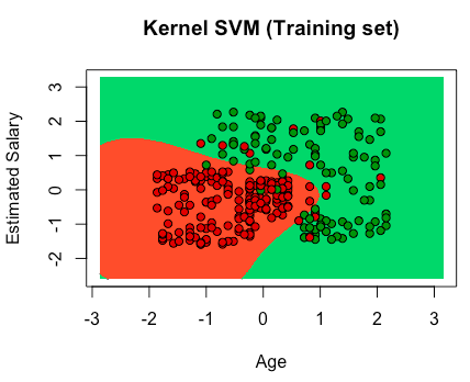
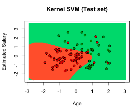
# Kernel SVM # Importing the dataset dataset = read.csv('Social_Network_Ads.csv') dataset = dataset[3:5] # Encoding the target feature as factor dataset$Purchased = factor(dataset$Purchased, levels = c(0, 1)) # Splitting the dataset into the Training set and Test set # install.packages('caTools') library(caTools) set.seed(123) split = sample.split(dataset$Purchased, SplitRatio = 0.75) training_set = subset(dataset, split == TRUE) test_set = subset(dataset, split == FALSE) # Feature Scaling training_set[-3] = scale(training_set[-3]) test_set[-3] = scale(test_set[-3]) # Fitting classifier to the Training set # install.packages('e1071') library(e1071) classifier = svm(formula = Purchased ~ ., data = training_set, type = 'C-classification', kernel = 'radial') # Predicting the Test set results y_pred = predict(classifier, newdata = test_set[-3]) # Making the Confusion Matrix cm = table(test_set[, 3], y_pred) # Visualising the Training set results library(ElemStatLearn) set = training_set X1 = seq(min(set[, 1]) - 1, max(set[, 1]) + 1, by = 0.01) X2 = seq(min(set[, 2]) - 1, max(set[, 2]) + 1, by = 0.01) grid_set = expand.grid(X1, X2) colnames(grid_set) = c('Age', 'EstimatedSalary') y_grid = predict(classifier, newdata = grid_set) plot(set[, -3], main = 'Kernel SVM (Training set)', xlab = 'Age', ylab = 'Estimated Salary', xlim = range(X1), ylim = range(X2)) contour(X1, X2, matrix(as.numeric(y_grid), length(X1), length(X2)), add = TRUE) points(grid_set, pch = '.', col = ifelse(y_grid == 1, 'springgreen3', 'tomato')) points(set, pch = 21, bg = ifelse(set[, 3] == 1, 'green4', 'red3')) # Visualising the Test set results library(ElemStatLearn) set = test_set X1 = seq(min(set[, 1]) - 1, max(set[, 1]) + 1, by = 0.01) X2 = seq(min(set[, 2]) - 1, max(set[, 2]) + 1, by = 0.01) grid_set = expand.grid(X1, X2) colnames(grid_set) = c('Age', 'EstimatedSalary') y_grid = predict(classifier, newdata = grid_set) plot(set[, -3], main = 'Kernel SVM (Test set)', xlab = 'Age', ylab = 'Estimated Salary', xlim = range(X1), ylim = range(X2)) contour(X1, X2, matrix(as.numeric(y_grid), length(X1), length(X2)), add = TRUE) points(grid_set, pch = '.', col = ifelse(y_grid == 1, 'springgreen3', 'tomato')) points(set, pch = 21, bg = ifelse(set[, 3] == 1, 'green4', 'red3')) |