Machine Learning A-Z: Part 2 – Regression (Decision Tree Regression)
Decision Tree Intuition
CART (Classification and Regression Trees)
– Classification Trees
– Regression Trees
Splitting data into segments.
Split 1: X1 < 20
Split 2: X2 < 200
Split 3: X2 < 170
Split 4: X1 < 40
Decision Tree Regression
Python
|
1 2 3 4 5 6 7 8 9 10 11 12 13 14 15 16 17 18 19 20 21 22 23 24 25 26 27 28 29 30 31 32 33 34 35 36 37 38 39 40 41 42 43 44 45 46 47 48 49 |
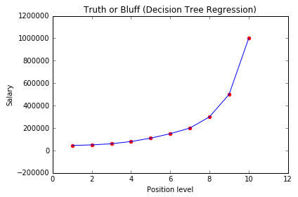
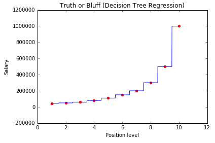
# Decision Tree Regression # Importing the libraries import numpy as np import matplotlib.pyplot as plt import pandas as pd # Importing the dataset dataset = pd.read_csv('Position_Salaries.csv') X = dataset.iloc[:, 1:2].values y = dataset.iloc[:, 2].values # Splitting the dataset into the Training set and Test set """from sklearn.cross_validation import train_test_split X_train, X_test, y_train, y_test = train_test_split(X, y, test_size = 0.2, random_state = 0)""" # Feature Scaling """from sklearn.preprocessing import StandardScaler sc_X = StandardScaler() X_train = sc_X.fit_transform(X_train) X_test = sc_X.transform(X_test) sc_y = StandardScaler() y_train = sc_y.fit_transform(y_train)""" # Fitting the Decision Tree Regression to the dataset from sklearn.tree import DecisionTreeRegressor regressor = DecisionTreeRegressor(random_state = 0) regressor.fit(X, y) # Predicting a new result y_pred = regressor.predict(6.5) # Visualizing the Decision Tree Regression results plt.scatter(X, y, color = 'red') plt.plot(X, regressor.predict(X), color = 'blue') plt.title('Truth or Bluff (Decision Tree Regression)') plt.xlabel('Position level') plt.ylabel('Salary') plt.show() # Visualising the Decision Tree Regression results (for higher resolution and smoother curve) X_grid = np.arange(min(X), max(X), 0.01) X_grid = X_grid.reshape((len(X_grid), 1)) plt.scatter(X, y, color = 'red') plt.plot(X_grid, regressor.predict(X_grid), color = 'blue') plt.title('Truth or Bluff (Decision Tree Regression)') plt.xlabel('Position level') plt.ylabel('Salary') plt.show() |
R
|
1 2 3 4 5 6 7 8 9 10 11 12 13 14 15 16 17 18 19 20 21 22 23 24 25 26 27 28 29 30 31 32 33 34 35 36 37 38 39 40 41 42 43 44 45 46 47 48 49 50 51 52 53 54 |
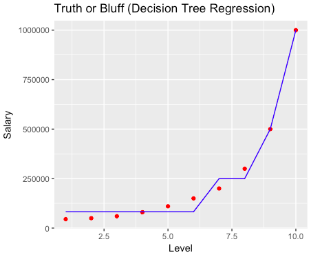
# Decision Tree Regression # Importing the dataset dataset = read.csv('Position_Salaries.csv') dataset = dataset[2:3] # Splitting the dataset into the Training set and Test set # install.packages('caTools') # library(caTools) # set.seed(123) # split = sample.split(dataset$DependentVariable, SplitRatio = 0.8) # training_set = subset(dataset, split == TRUE) # test_set = subset(dataset, split == FALSE) # Feature Scaling # training_set = scale(training_set) # test_set = scale(test_set) # Fitting the Decision Tree Regression to the dataset # install.packages('rpart') # library(rpart) regressor = rpart(formula = Salary ~ ., data = dataset, control = rpart.control(minsplit = 1)) # Predicting a new result y_pred = predict(regressor, data.frame(Level = 6.5)) # Visualising the Decision Tree Regression results # install.packages('ggplot2') library(ggplot2) ggplot() + geom_point(aes(x = dataset$Level, y = dataset$Salary), color = 'red') + geom_line(aes(x = dataset$Level, y = predict(regressor, newdata = dataset)), color = 'blue') + ggtitle('Truth or Bluff (Decision Tree Regression)') + xlab('Level') + ylab('Salary') # Visualising the Decision Tree Regression results (for higher resolution and smoother curve) # install.packages('ggplot2') # library(ggplot2) x_grid = seq(min(dataset$Level), max(dataset$Level), 0.1) ggplot() + geom_point(aes(x = dataset$Level, y = dataset$Salary), color = 'red') + geom_line(aes(x = x_grid, y = predict(regressor, newdata = data.frame(Level = x_grid))), color = 'blue') + ggtitle('Truth or Bluff (Decision Tree Regression)') + xlab('Level') + ylab('Salary') |