Python Tools
Adjusted Closing Price
Adjusted Closing Price
http://www.investopedia.com/terms/a/adjusted_closing_price.asp
How do I calculate the adjusted closing price for a stock?
http://www.investopedia.com/ask/answers/06/adjustedclosingprice.asp
Data Analysis and Visualization: Stock Market Analysis
Reference
Moving Average – MA
http://www.investopedia.com/terms/m/movingaverage.asp
How To Use A Moving Average To Buy Stocks
http://www.investopedia.com/articles/active-trading/052014/how-use-moving-average-buy-stocks.asp
Pearson correlation coefficient
http://en.wikipedia.org/wiki/Pearson_product-moment_correlation_coefficient
Annotating Axes: matplotlib
http://matplotlib.org/users/annotations_guide.html
Quantile
https://en.wikipedia.org/wiki/Quantile
Monte Carlo Simulation With GBM
http://www.investopedia.com/articles/07/montecarlo.asp
The Rate of Return of Amazon’s Stock Price
|
1 2 3 4 5 6 7 |
import numpy as np from pandas_datareader import data as wb import matplotlib.pyplot as plt AMZN = wb.DataReader('AMZN', data_source='google', start='2000-1-1') AMZN.head() |
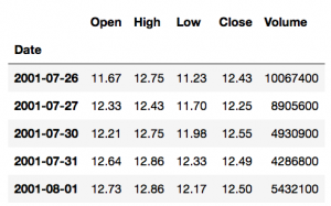
|
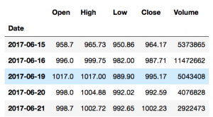
1 |
AMZN.tail() |
|
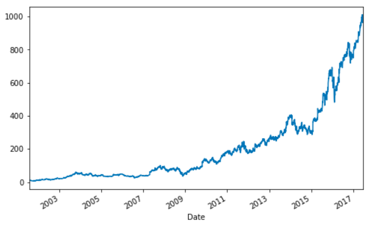
1 2 |
AMZN['Close'].plot(figsize=(8,5)) plt.show() |
Simple rate of return
rate of return = (ending price – beginning price) / beginning price
(P1 – P0) / P0 = P1 / P0 – 1
Use when dealing with multiple assets over the same timeframe.
|
1 2 |
AMZN['simple_return'] = (AMZN['Close'] / AMZN['Close'].shift(1)) - 1 print (AMZN['simple_return']) |
Date
2001-07-26 NaN
2001-07-27 -0.014481
2001-07-30 0.024490
2001-07-31 -0.004781
2001-08-01 0.000801
2001-08-02 -0.024800
2001-08-03 -0.003281
2001-08-06 -0.020576
2001-08-07 -0.025210
2001-08-08 -0.042241
2001-08-09 -0.058506
2001-08-10 -0.048757
2001-08-13 0.017085
2001-08-14 0.040514
2001-08-15 -0.042735
2001-08-16 -0.026786
2001-08-17 0.018349
2001-08-20 0.041041
2001-08-21 -0.049038
2001-08-22 0.031345
2001-08-23 -0.055882
2001-08-24 0.062305
2001-08-27 -0.009775
2001-08-28 -0.015795
2001-08-29 -0.078235
2001-08-30 -0.054407
2001-08-31 0.028769
2001-09-04 -0.039150
2001-09-05 -0.109430
2001-09-06 0.065359
…
2017-05-10 -0.004062
2017-05-11 -0.001402
2017-05-12 0.014489
2017-05-15 -0.003516
2017-05-16 0.008455
2017-05-17 -0.022058
2017-05-18 0.014533
2017-05-19 0.001408
2017-05-22 0.011283
2017-05-23 0.000896
2017-05-24 0.009068
2017-05-25 0.013291
2017-05-26 0.002416
2017-05-30 0.000924
2017-05-31 -0.002087
2017-06-01 0.001337
2017-06-02 0.010824
2017-06-05 0.004579
2017-06-06 -0.008246
2017-06-07 0.007049
2017-06-08 0.000198
2017-06-09 -0.031635
2017-06-12 -0.013697
2017-06-13 0.016457
2017-06-14 -0.004405
2017-06-15 -0.012596
2017-06-16 0.024415
2017-06-19 0.007553
2017-06-20 -0.002593
2017-06-21 0.009712
Name: simple_return, Length: 4000, dtype: float64
|
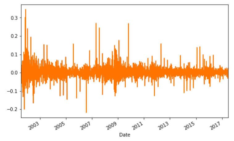
1 2 |
AMZN['simple_return'].plot(figsize=(8,5)) plt.show() |
|
1 2 |
avg_returns_d = AMZN['simple_return'].mean() avg_returns_d |
0.0015193424705951424
|
1 2 |
avg_returns_a = AMZN['simple_return'].mean() * 250 avg_returns_a |
0.3798356176487856
|
1 |
print (str(round(avg_returns_a, 5) * 100) + ' %') |
37.984 %
Logarithmic rate of return
ln(Pt / Pt-1)
10.0% = log $116 / $105 = log $116 – log $105
Use when you make calculations about a single asset over time.
|
1 2 |
AMZN['log_return'] = np.log(AMZN['Close'] / AMZN['Close'].shift(1)) print (AMZN['log_return']) |
Date
2001-07-27 NaN
2001-07-30 0.024195
2001-07-31 -0.004792
2001-08-01 0.000800
2001-08-02 -0.025113
2001-08-03 -0.003287
2001-08-06 -0.020791
2001-08-07 -0.025533
2001-08-08 -0.043159
2001-08-09 -0.060287
2001-08-10 -0.049986
2001-08-13 0.016941
2001-08-14 0.039715
2001-08-15 -0.043675
2001-08-16 -0.027151
2001-08-17 0.018182
2001-08-20 0.040221
2001-08-21 -0.050282
2001-08-22 0.030864
2001-08-23 -0.057504
2001-08-24 0.060441
2001-08-27 -0.009823
2001-08-28 -0.015921
2001-08-29 -0.081465
2001-08-30 -0.055943
2001-08-31 0.028363
2001-09-04 -0.039937
2001-09-05 -0.115893
2001-09-06 0.063312
2001-09-07 0.043224
…
2017-05-11 -0.001403
2017-05-12 0.014385
2017-05-15 -0.003522
2017-05-16 0.008420
2017-05-17 -0.022305
2017-05-18 0.014428
2017-05-19 0.001407
2017-05-22 0.011220
2017-05-23 0.000896
2017-05-24 0.009027
2017-05-25 0.013204
2017-05-26 0.002413
2017-05-30 0.000923
2017-05-31 -0.002089
2017-06-01 0.001336
2017-06-02 0.010766
2017-06-05 0.004569
2017-06-06 -0.008281
2017-06-07 0.007024
2017-06-08 0.000198
2017-06-09 -0.032146
2017-06-12 -0.013792
2017-06-13 0.016324
2017-06-14 -0.004414
2017-06-15 -0.012676
2017-06-16 0.024122
2017-06-19 0.007524
2017-06-20 -0.002596
2017-06-21 0.009665
2017-06-22 -0.000928
Name: log_return, dtype: float64
|
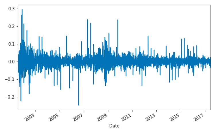
1 2 |
AMZN['log_return'].plot(figsize=(8, 5)) plt.show() |
|
1 2 |
log_return_d = AMZN['log_return'].mean() log_return_d |
0.0010977419081520047
|
1 2 |
log_return_a = AMZN['log_return'].mean() * 250 log_return_a |
0.2744354770380012
|
1 |
print (str(round(log_return_a, 5) * 100) + ' %') |
27.444 %